Computing Cortical and Trabecular Measurements
Global and per slice measurements of common bone morphometric indices, as described by Bouxsein et al*, can be computed automatically from segmented trabecular and cortical bone.
Options for automatically segmenting cortical and trabecular areas, as well as for computing global measurements (see Computing Global Measurements), are available in the Bone Analysis dialog, shown below. Results can be output in comma-separated values files (*.csv extension).
Bone Analysis dialog

In addition to the global measurements available for bone morphometric indices, per slice measurements in any oblique for segmented areas (see Computing Slice-by-Slice Measurements) are available in the Slice Analysis dialog, shown below. The input for computing slice-by-slice measurements can be any region of interest — segmented bone, cortical bone, or trabeculae. Results can be output in comma-separated values files (*.csv extension).
Slice Analysis dialog

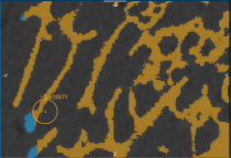
Closing the holes in an initial bone segmentation, including cortical pores and vascular canal inlets, and filling the inner areas of the segmentation, is the first step in the bone analysis workflow for accurately quantifying morphometric indices.
Cortical pore (circled)

The output of this process is a filled region of interest, which is an input for separating cortical and trabecular bone.
and a filled region of interest in which the holes of the bone segmentation are closed.
Region of interest (Filled)… The segmentation of the filled area corresponding to the bone cortex and the marrow.
- Create and refine a region of interest in which the sample's mineralized bone is labeled (see Performing Initial Bone Segmentations and Refining Initial Bone Segmentations).
- Make sure that the region of interest is sealed on all sides (see Sealing an Initial Bone Segmentation).
- Choose Tools > Bone Analysis on the menu bar to open the Bone Analysis dialog.
- Select the region of interest that you want to fill in the Bone drop-down menu.
- Enter the required threshold distance to close the cortical pores and vascular canal inlets in the Close holes smaller than edit box.

- Click the Fill button to start the automated routine.

- Wait for the process to be completed.
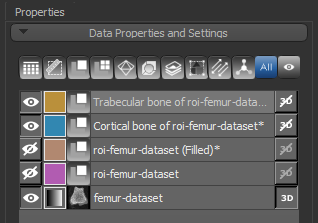
At the end of the process, a new region of interest (Filled) will appear in the Data Properties and Settings panel.

- Verify the accuracy of the result, recommended.

- Edit the filled region of interest, if required.
See ROI Painter Tools and other topics in Segmentation for information about the segmentation tools available in Dragonfly for editing ROIs.
- Click Next to continue to the next segmentation step.


Segmentation of the cortical and trabecular bone is the most critical step for the accurate quantification of selected morphometric indices. Two methods — Kohler and Buie — are available for segmenting cortical and trabecular bone. The input of the automated segmentation is a bone segmentation in which bone mineralization is present (see Performing Initial Bone Segmentations) and a filled region of interest in which the bone segmentation are filled. The output of the process is two regions of interest listed below:
Cortical bone… The intersection of the cortical area with the input bone segmentation.
Trabecular bone… The intersection of the trabecular area with the input bone segmentation.
|
|
Description |
|---|---|
|
Segmentation method |
Two methods — Kohler and Buie — are available for segmenting cortical and trabecular bone. Kohler… This segmentation method relies on basic image processing concepts using morphological and other operators to separate cortical from trabecular bone. Refer to Kohler et el, Automated compartmental analysis for high-throughput skeletal phenotyping in femora of genetic mouse models, Bone, 41, 4, (659-667), (2007) for details about this method. NOTE In general, the Kohler method works best on single, regularly-shaped bone specimens. In addition, the initial bone segmentation must be closed on all sides (see Refining Initial Bone Segmentations). Buie… This dual threshold method to segment bone regions usually produces accurate and repeatable results. Refer to Buie et al, Automatic segmentation of cortical and trabecular compartments based on a dual threshold technique for in vivo micro-CT bone analysis, Bone, 41, 4, (505-515), (2007) for details about this method. |
|
Trabecular thickness |
The expected maximal thickness of the trabeculae RECOMMENDATIONS You can measure trabecular thickness with the Ruler tool (see Using the Ruler Tool) or you can generate a thickness mesh from a sub-sample of the trabeculae and then find the maximum thickness of the mesh by computing a histogram (see Exporting ROIs and Multi-ROI Classes to Thickness Meshes). |
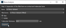
- Make sure that you are on the Separation of the filled bone as cortical and trabecular bone screen of the Bone Analysis dialog.
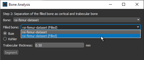
- Select the region of interests that will provide the inputs for segmenting cortical and trabecular bone in the Bone and Filled bone drop-down menus.

You can select the filled region of interest you created in the previous step, an edited region of interest, or any other region of interest that satisfies the required criteria.
- Choose a segmentation method — Kohler or Buie — to segment cortical and trabecular bone.
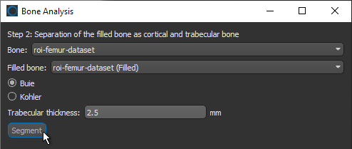
- Enter the expected maximal thickness of the trabeculae in the Trabecular thickness edit box.
- Click the Segment button to start the automated segmentation routine.
If you selected the Kohler method, use the slider to select a threshold to separate the cortical and trabecular bone.

- Wait for the automated segmentation to be completed.
At the end of the process, two new regions of interest — Cortical bone and Trabecular bone — appear in the Data Properties and Settings panel.
- Verify the accuracy of the cortical and trabecular bone segmentations, recommended.
- Verify the accuracy of the result, recommended.

- Edit the regions of interest, if required (see Editing Automated Segmentations).
- Click Next to continue to the next segmentation step.

In some cases, an automated segmentation may result in voxels corresponding to trabecular bone erroneously labeled as cortical bone, as circled below, or vice versa.
Automated segmentation result

To edit a segmentation, you can automatically re-assign labeled voxels from one region to interest to another with the Brush tools (see Working with the ROI Painter Tools in 2D Views). In addition, when you work in the Exclusive mode with the Brush tools, only the labeled voxels belonging to the selected regions of interest will be affected when painting.
- Select the 2D view in which you plan to edit the regions of interest.
- Select the two regions of interest in the Data Properties and Settings panel.
If you want to re-assign voxels labeled as cortical bone to those labeled as trabecular bone, make sure that the trabecular bone ROI is identified as (A) and that the cortical bone ROI is identified as (B).
- Select a 2D Brush or 3D Brush on the ROI Painter panel.
- Select the Exclusive option, circled below.

NOTE In this mode, painting will only be applied to the labeled voxels of the selected regions of interest. Unlabeled voxels will not be painted.
- Do the following, as required:
- Re-assign labeled voxels to ROI (A) from ROI (B) by holding down Left Ctrl (or your configured Add with key) and then painting.
- Re-assign labeled voxels from ROI (A) to ROI (B) by holding down Left Shift (or you configured Remove with key) and then painting.
- Re-assign labeled voxels to ROI (A) from ROI (B) by holding down Left Ctrl (or your configured Add with key) and then painting.

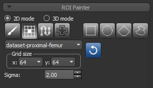
You can use the Smart Grid tool, as described below, or any other manual ROI Painter Tool to re-assign labeled voxels from one region of interest to another (see ROI Painter Tools).
- Select the 2D view in which you plan to edit the region of interest.
- Click the Smart Grid
 tool on the ROI Painter panel.
 - Select the dataset you are working with in the drop-down menu and then adjust the grid size, as required (see Working with the ROI Painter Tools in 2D Views).
- Select the region of the interest with the labeled voxels you need to re-assign in the Data Properties and Settings panel.
- Remove mislabeled voxels from the region of interest by holding down Left Shift (or your configured Remove by key) and then painting within the grid lines.

- Select the region of interest to which you want to add voxels.
- Add voxels to the required region of interest by holding down Left Ctrl (or your configured Add by key) and then painting within the grid lines.

- Scroll through the image slices and continue to refine the segmented regions, as required.


Segmented cortical and trabecular areas drive the computation of measurements, described below, for the common bone morphometric indices that provide quantitative descriptions of bone micro-architecture.
|
Abbr. |
Measurement |
Description |
|---|---|---|
|
Ani.MIL |
Anisotropy (MIL)* |
A measurement of the orientation of trabecular architecture computed with the Mean Intercept Length (MIL) method, which uses the mean distance between material intersections (bone–marrow interfaces) along linear traverses over a range of orientations. Because MIL traverses cross both materials, the result is a combined measure that incorporates features of both materials. Refer to W.J. Whitehouse, The quantitative morphology of anisotropic trabecular bone, Journal of Microscopy, 101, 2, (153–168), (1974) for more information about the MIL method. |
|
Ani.SVD |
Anisotropy (SVD)* |
A measurement of the orientation of trabecular architecture that uses the Star Volume Distribution (SVD) method. In this method, the distribution is determined by placing a series of points within the material of interest, and then measuring the lengths of the lines emanating from them in various directions until they encounter a boundary. These lines are considered infinitesimal cones, with their vertex at the origin and subtending a solid angle as they approach the material interface. Refer to L.M. Cruz-Orive, L.M. Karlsson, S.E. Larsen, F. Wainschtein, Characterizing anisotropy: A new concept, Micron and Microscopica Acta, 23, (75-76), (1992) for more information about the SVD method. |
|
TV |
Total volume |
The volume of the segmented cortical and marrow (trabecular) areas that were computed from the input bone segmentation. |
|
BV |
Bone volume |
The volume of cortical and trabecular bone that were computed from the input bone segmentations. |
|
BV/TV |
Bone volume fraction |
The ratio of the bone volume (BV) to the total volume (TV). NOTE Several studies show that the degree of anisotropy, a description of how the structural elements are oriented, together with bone volume fraction may explain a significant part of the mechanical properties of a 3D structure. |
|
Ct.Th |
Average cortical thickness |
The mean thickness of cortical bone, assessed using direct 3D methods. NOTE Calculated by fitting maximal spheres within the cortical structure. |
|
Tb.Th |
Average trabecular thickness |
The mean thickness of trabeculae, assessed using direct 3D methods. NOTE Calculated by fitting maximal spheres within the trabecular structure. |
|
Tb.Sp |
Average trabecular separation |
The mean distance between trabeculae, assessed using direct 3D methods. Tb.Sp is sometimes called trabecular spacing. NOTE Higher Tb.Sp is associated with vertebral fracture and generally increases with age, exhibiting a linear dependence on age in the lumbar spine. |
|
Ct.Ar |
Average cortical area |
The mean cortical bone area, which is computed as: |
|
Ma.Ar |
Average marrow area |
The mean medullary (or marrow) area, which is computed as: NOTE Treatments that tend to increase total cross-sectional area Tt.Ar and cortical area Ct.Ar can lead to a decrease in Ma.Ar, as an increase in bone area also increases the ratio of cortical to medullary bone. |
|
Tt.Ar |
Average total area |
The total cross-sectional area inside the periosteal envelope, measured for each transverse section. NOTE Tt.Ar has been found to increase with age with continued periosteal apposition in both men and women at the distal radius and distal tibia. Cross-sectional area measurements characterize resistance to axial compression and tension. |
|
Ct.Ar/Tt.Ar |
Average cortical area fraction |
The ratio of the mean cortical area to the mean total area. |
|
Ps.S3D |
Periosteal surface (3D) |
The total surface area of the periosteum, which is the membrane that lines the outer surface of all bones, except at the joints of long bones. |
|
Ec.S3D |
Endocortical surface (3D) |
The total surface area of the endocortex, which lines the inner surface of all bones. |
|
Ps.Pm |
Periosteal perimeter |
The total perimeter of the periosteum. |
|
Ec.Pm |
Endocortical perimeter |
The total perimeter of the endocortex. |
* The degree of anisotropy, computed using with the MIL or SVD method, is a measure of how highly oriented substructures are within a volume. Trabecular bone varies its orientation depending on mechanical load and can become anisotropic. For an isotropic (perfectly oriented) system, the degree of anisotropy (DA) is equal to 0. As the system becomes more anisotropic (less well-oriented), the DA increases to some value less than or equal to 1.
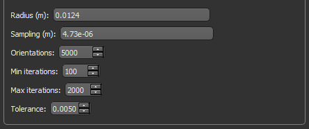
Refer to the table below for the settings applicable to anisotropy computations.
|
|
Description |
|---|---|
|
Radius (m) |
The radius of the sampling sphere, which determines the length of each sampling vector |
|
Sampling (m) |
The resolution, or distance between subsequent samples along each vector RECOMMENDATIONS You can accept the default value or enter a value can be equal to the voxel size of the input region of interest. |
|
Orientations |
The number of lines to analyze per sampling sphere |
|
Min iterations |
The minimum number of random points in the sample that will be analyzed. |
|
Max iterations |
Is the maximum number of random points in the sample that will be analyzed. Fitting will stop automatically after this number is completed or if the coefficient of variation (tolerance) is reached. |
|
Tolerance |
The coefficient of variation. Sampling new random points will continue until either a coefficient of variation equal to the tolerance is reached or the set maximum number of iterations is completed. |
Refer to the following publications for additional information:
- Segment the cortical and trabecular bone in your sample (see Segmenting Cortical and Trabecular Bone).
- On the Compute global measurements screen of the Bone Analysis dialog, select the region of interest that represents the filled cortical and marrow (trabecular) areas in the Filled bone drop-down menu.
NOTE You can select the filled region of interest you created previously, an edited region of interest, or any other region of interest that satisfies the required criteria.
- Select the regions of interest that represent the segmented cortical and trabecular bone in the Cortical bone and Trabecular bone drop-down menus.

NOTE You can select the regions of interest that you created previously, edited regions of interest, or any other regions of interest that satisfy the required criteria.
- Do one of the following for Trabecular thickness:
- If you selected the regions of interest you created during the Bone Analysis workflow for computing global measurements, the value you entered previously will appear in the edit box. You can keep this value or adjust it, if required. For example, if you plan to compute indices such as bone volumes and areas.
- If you selected new regions of interest as your inputs, enter the expected maximal thickness of the trabeculae.
- Select measurements that you want to compute.
NOTE If you are computing anisotropy with the MIL or SVD method, you will need to select the required settings, which are available at the bottom of the dialog (see Settings for Computing Anisotropy).
- Click the Compute measurements button at the bottom of the dialog.
The selected measurements are computed and appear in the Bone Analysis dialog.
- Click the Export to CSV button to export your results in a comma-separated values file (*.csv extension), optional.
NOTE The delimiter for exporting in the CSV file format — comma, semicolon, or tab — can be selected in the Preferences dialog (see Miscellaneous Preferences).

In addition to the global measurements available for bone morphometric indices, per slice measurements in any oblique for segmented bone, cortical bone, and trabeculae are available in the Slice Analysis dialog. The available measurements for applicable regions of interest are described in the table below.
|
Measurement |
Description |
|---|---|
|
Voxel Count |
The total number of voxels contained in the selected region of interest. |
|
Moments of inertia |
Available for any oblique of interest, such as the normal to the direction of the bone shaft, the moments of inertia listed below can be extracted from an initial bone segmentation.
Ixx… The moment of inertia around the X axis, which is a measure of how material is distributed about the axis through the area centroid of each slice. Area moments of inertia are also known as second moments of area and characterize resistance to bending around a given axis. Iyy… The moment of inertia around the Y axis, which is a measure of how material is distributed about the axis through the area centroid of each slice. Area moments of inertia are also known as second moments of area and characterize resistance to bending around a given axis. Imax… The maximum moment of inertia, which is a measure of how material is distributed about the major centroidal axis, which is orthogonal to the minor centroidal axis. The maximum moment of inertia correlates to the maximum bending strength of a bone. Area moments of inertia are also known as second moments of area and characterize resistance to bending around a given axis. Imin… The minimum moment of inertia, which is a measure of how material is distributed about the minor centroidal axis, which is orthogonal to the major centroidal axis. The minimum moment of inertia correlates to the minimum bending strength of a bone. Area moments of inertia are also known as second moments of area and characterize resistance to bending around a given axis. J… The polar moment of inertia, which is the sum of any two perpendicular area moments of inertia (Imax + Imin) and characterizes resistance to torsion. |
|
Th (mean thickness) |
Available for any oblique of interest, such as the normal to the direction of the bone shaft, the mean thickness can be extracted from segmented cortical or trabecular bone.
NOTE You can compute the average trabecular separation by creating a new region of interest in which the ROI of the trabecular bone is subtracted from the ROI of the trabecular area (see Applying Boolean Operations). |
|
Pm (perimeter) |
Available for any oblique of interest, such as the normal to the direction of the bone shaft, the periosteal and endocortical perimeters can be extracted from segmented cortical or trabecular areas, respectively.
In most cases, you should choose to fill the inner areas on the slices whenever you compute the periosteal or endocortical perimeter.
|
|
ROI Area |
The total area of the labeled voxels contained in the selected region of interest. |


- Segment the bone specimen, as required.
See Performing Initial Bone Segmentations and Segmenting Cortical and Trabecular Bone.
- Select the 2D view of the region of interest that you want to analyze.
You can adjust the orientation of the view, if required (see Creating Oblique Views).
- Right-click the required 2D view of the region of interest and then choose Start Slice Analysis in the pop-up menu.

The Slice Analysis panel appears on the right sidebar (see Analyzing Slices).
NOTE Slice Analysis panels are linked to the view in which they are accessed. This linking is indicated with the color-coded bar at the top of the panel. If required, you can open multiple panels to directly compare measurements between different views.
- Select the region of interest that you want to analyze in the Object studied drop-down menu, as shown below.

You should note the following:
- Moments of inertia are usually extracted from bone segmentations.
- Measurements of mean thickness (Th) are usually extracted separately from cortical and trabecular bone segmentations.
- Measurements of the periosteal perimeter can be extracted from cortical area segmentations.
- Measurements of the endocortical perimeter can be extracted from trabecular area segmentations.
- Choose a mask in the Mask drop-down menu if you want limit the computations to the sub-volume defined by a region of interest, optional.
Check the Use inverted mask option to compute measurements outside the selected mask.
- Select the measurement(s) that you want to compute.
NOTE If you are computing periosteal or endocortical perimeters, you can choose to fill the inner areas on the slices.
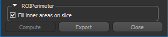
- Click the Compute button at the bottom of the panel.
The results appear in the Slice Analysis panel.
- Click the Export button to export your results in a comma-
- separated values file (*.csv extension), optional.
NOTE The delimiter for exporting in the CSV file format — comma, semicolon, or tab — can be selected in the Preferences dialog (see Miscellaneous Preferences).